LQG Lane-Keeping for an Autonomous Vehicle
For my final project in Advanced Computer Control (ME 462), I designed a controller that keeps a car centred in its lane at highway speed, using only the noisy measurements a real car would have. It's a solo project, written up as a full report: I derived the vehicle model, proved the design was valid, built a race-track test environment, and simulated everything in MATLAB.
The controller is LQG (Linear Quadratic Gaussian): an optimal steering law (LQR) paired with a Kalman filter that estimates what the sensors can't measure directly.
speed
loop
the 4th estimated
Modeling the car
I modeled the car as a bicycle: the two front wheels are lumped into one, and so are the two rear wheels. That's accurate enough when the car isn't rolling or pitching much. Rather than tracking where the car is on the map, the model tracks how far it is off the lane: its sideways offset and its heading relative to the road. The goal is to drive both to zero.
The state is the lateral error, heading error and their rates:
$$x = \begin{bmatrix} e_y & \dot e_y & e_\psi & \dot e_\psi \end{bmatrix}^\top$$Newton's second law for sideways motion and for yaw (rotation about the vertical axis):
$$m(\ddot y + V_x r) = F_{yf} + F_{yr}$$ $$I_z \dot r = l_f F_{yf} - l_r F_{yr}$$Below about 4° of slip, tire force is proportional to slip angle, \(F_y = C_\alpha \alpha\), with the slip angles coming from the geometry:
$$\alpha_f = \delta - \frac{\dot e_y + V_x e_\psi + l_f \dot e_\psi}{V_x}$$ $$\alpha_r = -\frac{\dot e_y + V_x e_\psi - l_r \dot e_\psi}{V_x}$$Substituting everything gives a linear model, with steering angle \(u = \delta\) as the input and road curvature as a disturbance \(w_d = V_x \kappa\):
$$\dot x = Ax + Bu + Ew_d$$For a 1500 kg mid-size sedan at 25 m/s, the numbers work out to:
$$A = \begin{bmatrix} 0 & 1 & 0 & 0 \\ 0 & -9.07 & 226.67 & -0.52 \\ 0 & 0 & 0 & 1 \\ 0 & -0.35 & 42.67 & -12.18 \end{bmatrix}$$ $$B = \begin{bmatrix} 0 & 106.67 & 0 & 85.33 \end{bmatrix}^\top$$Is the design even possible?
Before designing a controller, two questions need a yes. Can steering alone move the car to any state? And can the sensors we have (a lane camera for offset and heading, plus a gyro for yaw rate) reveal the one state they don't measure, sideways velocity?
Both come down to a rank test. With \(n = 4\) states and measurement matrix \(C\) picking out \(e_y\), \(e_\psi\) and \(\dot e_\psi\):
$$\operatorname{rank}\begin{bmatrix} B & AB & A^2B & A^3B \end{bmatrix} = 4$$ $$\operatorname{rank}\begin{bmatrix} C \\ CA \\ CA^2 \\ CA^3 \end{bmatrix} = 4$$Full rank on both, so the system is controllable (LQR applies) and observable (a Kalman filter can reconstruct \(\dot e_y\)).
Building a test track
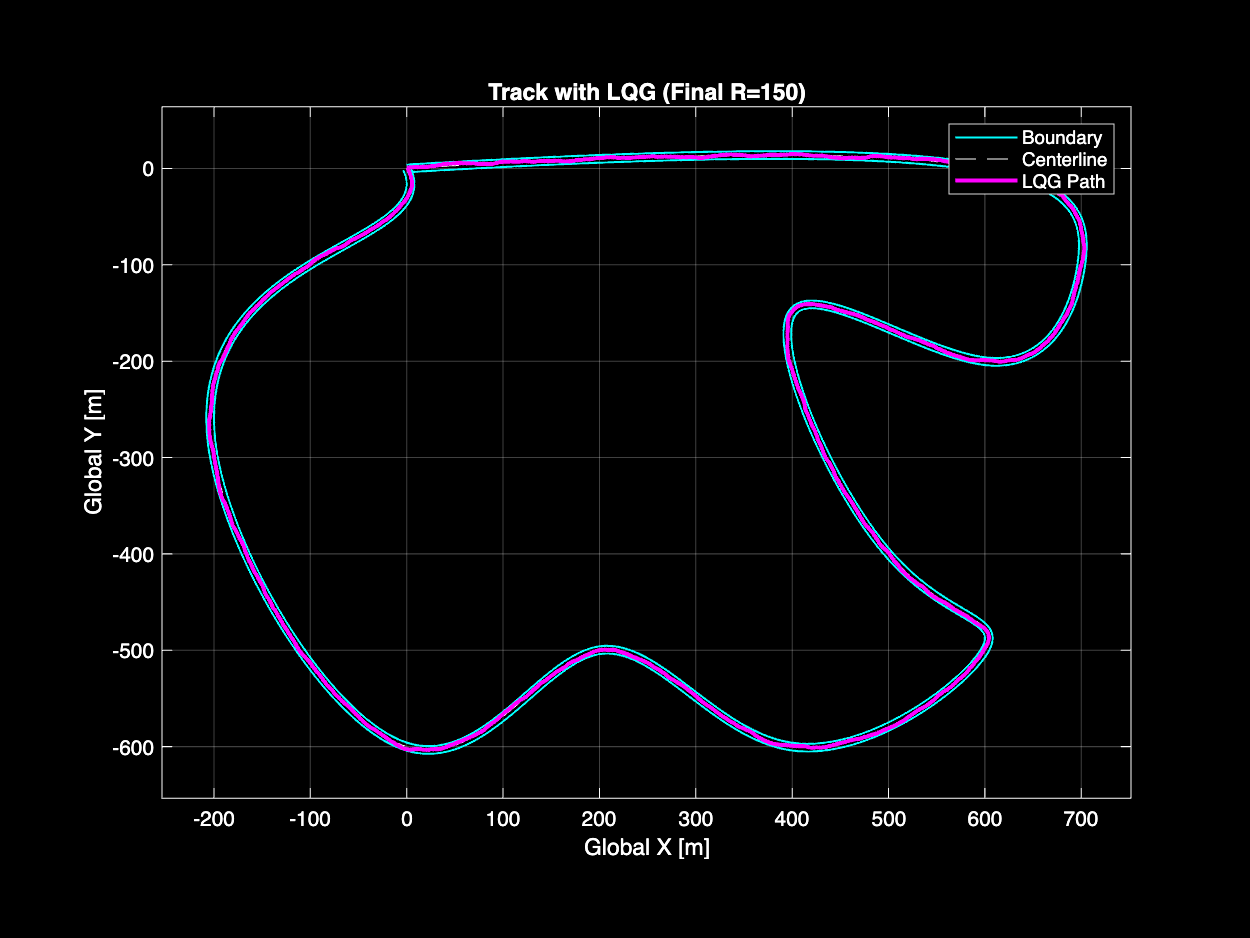
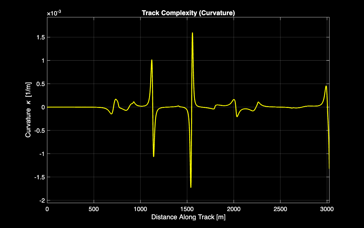
A straight road would be too easy a test. I built a closed circuit, loosely inspired by Bahrain, by fitting a cubic spline through hand-picked waypoints: long straights, hairpins and a chicane. Every bend shows up as a curvature spike that the controller has to react to.
For the spline \(P(s) = [x(s), y(s)]\), curvature is computed analytically instead of by finite differences:
$$\kappa(s) = \frac{x' y'' - y' x''}{\left(x'^2 + y'^2\right)^{3/2}}$$A Gaussian smoothing kernel (50 samples) is then applied, roughly mimicking how tires filter sharp changes in the road.
Steering optimally (LQR)
LQR finds the steering law that best balances two competing goals: stay close to the lane centre, and don't saw at the wheel. You choose how much each one matters, and the math returns the best feedback gains for that trade-off. On top of the feedback, a feedforward term pre-steers into each curve based on the road's curvature, so the feedback only has to clean up what's left.
LQR minimizes the infinite-horizon cost:
$$J = \sum_{k=0}^{\infty} \left( x_k^\top Q\, x_k + R\, u_k^2 \right)$$The optimal law is \(u_k = -Kx_k\), where \(K\) comes from the steady-state solution \(P\) of the discrete algebraic Riccati equation:
$$P = A_d^\top P A_d - A_d^\top P B_d \left(R + B_d^\top P B_d\right)^{-1} B_d^\top P A_d + Q$$ $$K = \left(R + B_d^\top P B_d\right)^{-1} B_d^\top P A_d$$For the final design I used \(Q = \mathrm{diag}(0.5,\ 0.1,\ 5,\ 0.1)\), weighting heading error most for directional stability, and a heavy \(R = 150\) on steering for a smooth, “limousine” ride. The feedforward term picks the steering that cancels the curvature disturbance at steady state:
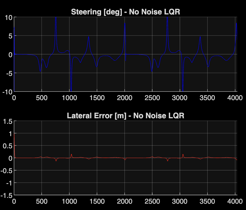
$$\delta_{ff} = -\left(B^\top B\right)^{-1} B^\top E \cdot V_x\, \kappa_{\text{road}}$$ $$u = -Kx + \delta_{ff}$$As a baseline, a more aggressive LQR (\(R = 15\)) with perfect, noise-free state knowledge tracks the lane almost exactly. Steering spikes only at the bends, and lateral error stays near zero after the initial 1 m offset is corrected.
Seeing the hidden state (Kalman filter)
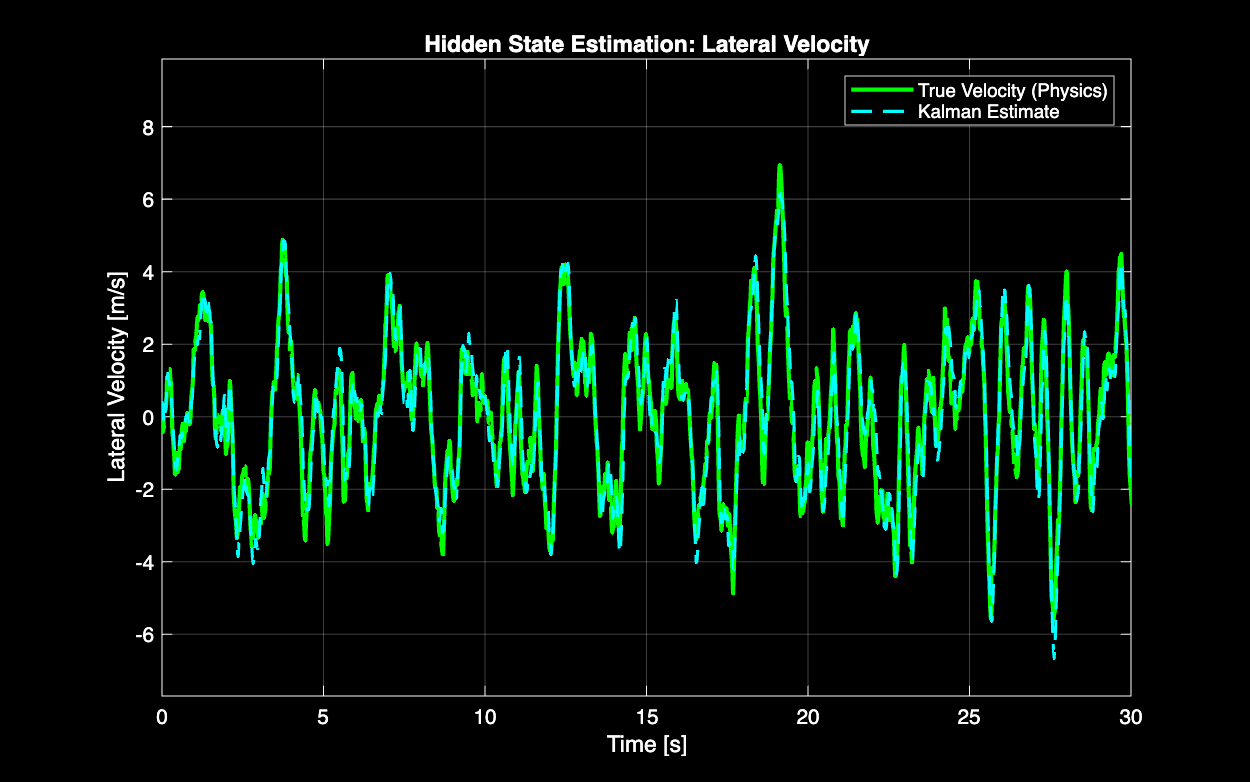
In reality the controller doesn't get perfect state. The camera and gyro are noisy, and no sensor measures sideways velocity at all. The Kalman filter runs the car model alongside the real car, predicts what the sensors should read, and corrects its estimate by however much they disagree, trusting each sensor according to how noisy it is.
The model is discretized with a zero-order hold at \(T_s = 0.02\) s (50 Hz), about 10× faster than the car's yaw dynamics. Each step, the filter predicts:
$$\hat x_{k|k-1} = A_d \hat x_{k-1} + B_d u_{k-1} + E_d w_k$$ $$P_{k|k-1} = A_d P_{k-1} A_d^\top + Q_{\text{est}}$$then corrects using the measurement \(y_k\):
$$L_k = P_{k|k-1} C^\top \left(C P_{k|k-1} C^\top + R_{\text{est}}\right)^{-1}$$ $$\hat x_k = \hat x_{k|k-1} + L_k\left(y_k - C\hat x_{k|k-1}\right)$$The sensor noise \(R_{\text{est}} = \mathrm{diag}(0.05^2,\ (1^\circ)^2,\ 0.01^2)\) corresponds to ±5 cm of lane offset, ±1° of heading and ±0.01 rad/s of gyro noise. The process noise \(Q_{\text{est}} = \mathrm{diag}(0.1,\ 1,\ 0.1,\ 1)\) puts more uncertainty on the rate states, standing in for wind and unmodeled tire behaviour.
Putting it together under noise
LQG simply feeds the Kalman estimate into the LQR gains. Thanks to the separation principle, the controller and the estimator can be designed independently and the combination stays stable. To see what the filter buys, I compared it against a “naive” LQR that plugs the noisy sensor readings straight into the aggressive baseline gains.
One caveat shaped the tuning. Pure LQR guarantees infinite gain margin and at least 60° of phase margin, but once an estimator is in the loop those guarantees vanish (Doyle's well-known counterexample). The heavy \(R = 150\) lowers the closed-loop bandwidth, which keeps the system away from the fast, unmodeled dynamics where robustness is weakest.
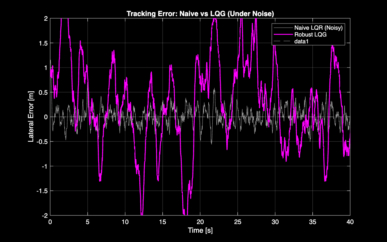
The result was a genuine trade-off rather than a clean win. The naive controller held lateral error within about ±0.5 m, but only by reacting to every bit of sensor noise with high-frequency steering. The LQG accepted larger excursions in the tight corners, up to about ±2 m, in exchange for smooth steering and stability that doesn't depend on clean measurements. Much of that gap comes from the tuning: the comfort weighting I chose for the LQG deliberately gives up some precision.
What I'd do next
The linear model is the main limitation. Tires saturate in hard cornering, so a nonlinear tire model (Pacejka's Magic Formula) would be the first upgrade. Speed was fixed at 25 m/s; braking into corners and scheduling the gains across speeds would shrink the corner errors. And since LQG can't enforce hard limits like “stay inside the lane”, model predictive control is the natural next step.