Differential Drive Robot — Full Autonomy Stack
Over a semester-long course project (ME 498, team of seven) we built a complete autonomy stack for a simulated two-wheeled robot, from the physics up. It started as a digital twin of the robot, then gained noisy sensors, a pose estimator and a feedback controller, and finally a planner that finds a path through obstacles and turns it into a smooth trajectory the robot can actually follow.
than raw GPS
than raw gyro
with moving obstacle
The page walks through the stack from the bottom up. I owned one core module in each phase — the dynamics, the pose estimator and the trajectory spline — marked My part below. Each section starts in plain English; the boxes underneath show the math for anyone who wants it.
Modeling the robot My part
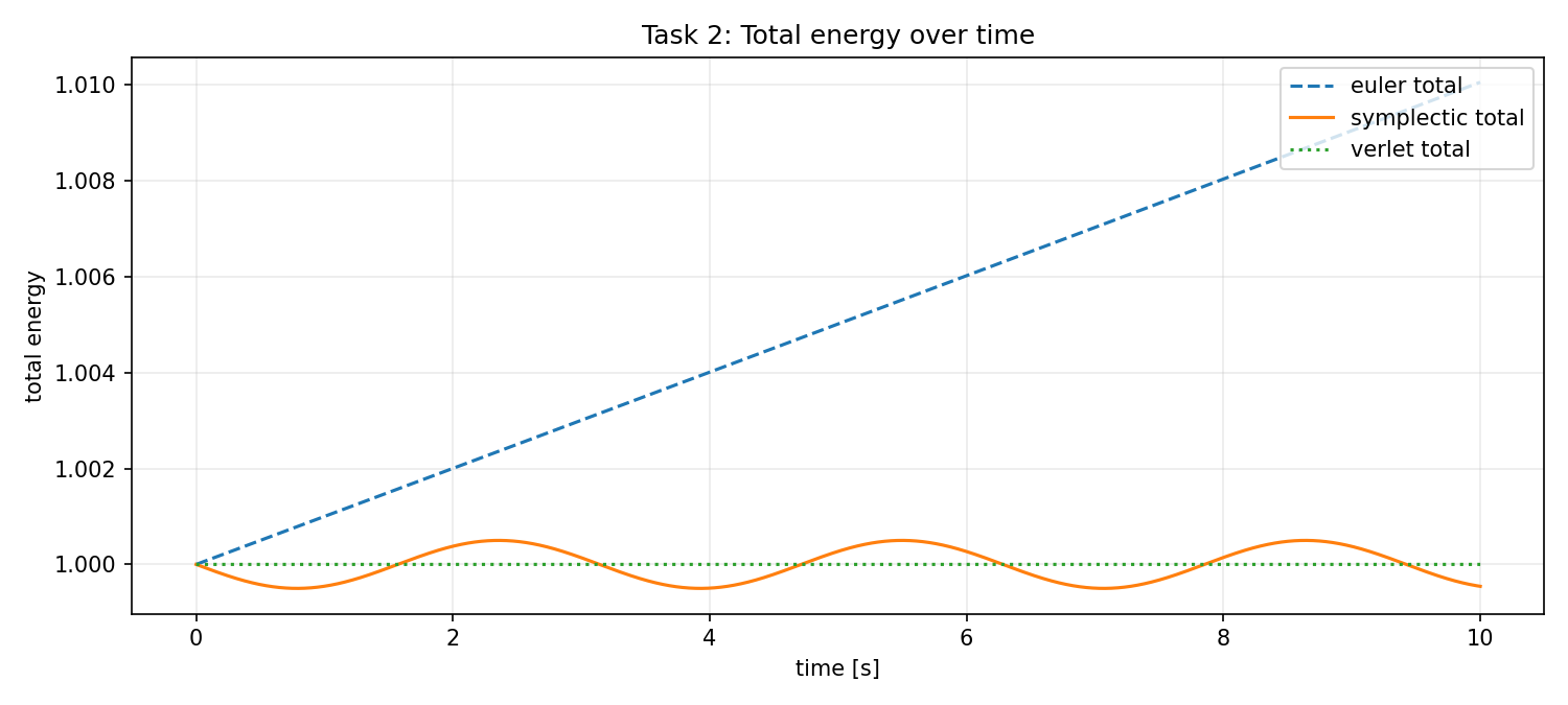
Everything else sits on top of a physics model, so it has to be right. The robot is a 2 kg body with two wheels that can each push forward or backward. Instead of tracking velocity, the simulator tracks momentum in the robot's own frame, which keeps the equations simple and makes energy behave properly over long runs.
The pose is \((x, y, \theta)\) and the body-frame momentum is \(p = (p_1, p_2, \ell)\). With mass matrix \(M = \mathrm{diag}(m, m, J)\), velocity is just \(w = M^{-1}p\), rotated into the world frame:
$$\begin{bmatrix}\dot x\\ \dot y\end{bmatrix} = R(\theta)\begin{bmatrix}v_1\\ v_2\end{bmatrix}, \qquad \dot\theta = \omega$$The wheel forces \(u_l, u_r\) (track width \(b\)) produce a forward push and a turning torque. Because the frame itself rotates, a Coriolis term appears in the momentum update:
$$\dot p = \underbrace{\begin{bmatrix} u_l + u_r \\ 0 \\ \tfrac{b}{2}(u_r - u_l)\end{bmatrix}}_{\text{wheels}} + F_{\text{ext}} + \underbrace{\begin{bmatrix} \omega\, p_2 \\ -\omega\, p_1 \\ 0 \end{bmatrix}}_{\text{rotating frame}}$$Leave out that last term and the robot quietly gains or loses energy every time it turns. The kinetic energy \(H = \tfrac12 p^\top M^{-1} p\) is the quantity we watched to check it.
Knowing where it is My part
The controller never sees the true pose — only noisy GPS, compass and gyro readings. GPS is noisy but doesn't drift; the gyro is smooth but drifts; the compass is unbiased but very noisy. The estimator combines them so each sensor covers for the others' weaknesses.
Position goes through a first-order low-pass filter (\(\alpha_x = 0.1\)):
$$\hat x_k = (1 - \alpha_x)\,\hat x_{k-1} + \alpha_x\, y^{\text{gps}}_k$$For white noise this shrinks the variance by a factor of \(\alpha/(2-\alpha) \approx 1/19\), about 4.4× less spread, at the cost of a few milliseconds of lag. Heading uses a complementary filter (\(\alpha_\theta = 0.02\)): integrate the gyro for short-term accuracy, then nudge toward the compass to cancel drift:
$$\hat\theta_k = (1 - \alpha_\theta)\big(\hat\theta_{k-1} + y^{\text{gyro}}_k\,\Delta t\big) + \alpha_\theta\, y^{\text{compass}}_k$$The estimate also exposes the rotation \(\hat Q = R(\hat\theta)\), which the controller uses to express tracking error in the robot's frame: \(e = \hat Q^\top (x^* - \hat x)\). Result: position error went from 0.142 m to 0.034 m, and heading error from 0.675 rad (gyro alone) to 0.052 rad.
Finding a path
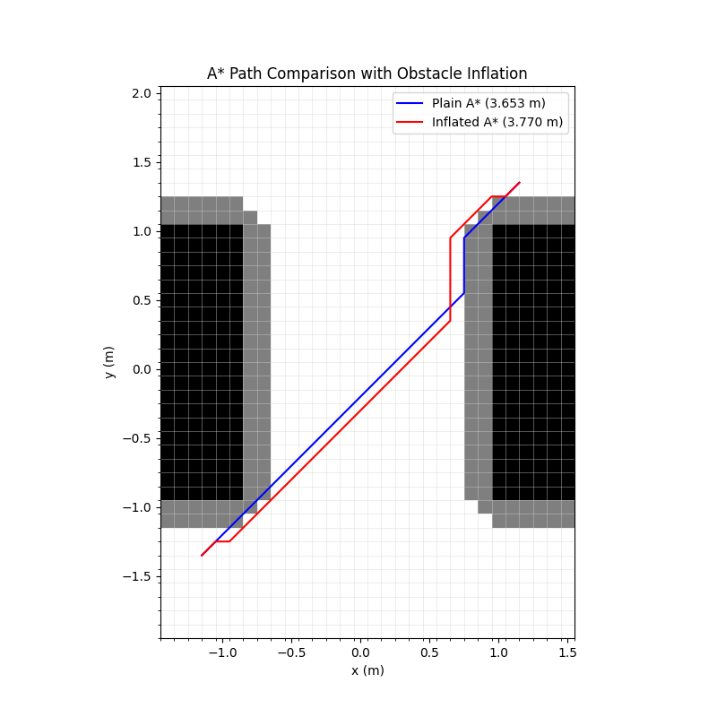
With the robot modeled and localized, the planner's job is to get it from start to goal. A* searches a grid of the map for the shortest collision-free route. Cells near obstacles are “inflated”: still allowed, but expensive, so the path keeps its distance unless squeezing past is really worth it.
A* always expands the cell with the lowest estimated total cost:
$$f(n) = g(n) + h(n), \qquad h(n) = \lVert n - n_{\text{goal}} \rVert_2$$\(g(n)\) is the cost so far: 1 for a straight step, \(\sqrt2\) for a diagonal, plus a penalty of 10 for entering an inflated cell. Since straight-line distance never overestimates the remaining cost, the heuristic is admissible and the path A* returns is optimal on the grid.
Smoothing it in time
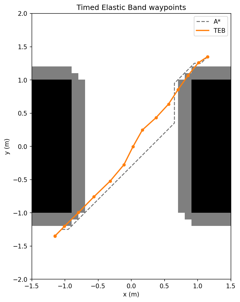
A grid path is jagged and says nothing about speed. A Timed Elastic Band takes the A* path as a starting guess and treats it like a rubber band: the waypoints and the time between them are free to move, pulled toward a path that is fast, smooth, clear of obstacles and under the 0.5 m/s speed limit.
The unknowns are the interior waypoints \(p_k\) and segment durations \(\Delta t_k\). With segment speed \(\bar v_k = \lVert p_{k+1} - p_k \rVert / \Delta t_k\) and distance to the nearest obstacle \(d_k\), the optimizer (L-BFGS-B) minimizes
$$\begin{aligned} J \;=\; &\gamma_t \textstyle\sum_k \Delta t_k \;+\; \gamma_s \textstyle\sum_k \lVert p_{k+1} - p_k \rVert^2 \\ +\; &\gamma_o \textstyle\sum_k \max(d_{\min} - d_k,\, 0)^2 \;+\; \gamma_v \textstyle\sum_k \max(\bar v_k - v_{\max},\, 0)^2 \\ +\; &\gamma_{bc}\big(\bar v_0^2 + \bar v_{N-1}^2\big) \end{aligned}$$Time, smoothness, clearance, speed limit, and starting/stopping at rest. The penalties are soft, so after solving, any waypoint inside \(d_{\min} = 0.15\) m is projected back out and any too-fast segment is slowed, turning them into hard guarantees.
A trajectory the robot can follow My part
The band gives a list of timed waypoints, but a controller can't track a list of points. Connect them with straight lines and the velocity jumps at every corner, which asks the motors for infinite acceleration. I built a cubic spline that threads a smooth curve through every waypoint, with continuous velocity and acceleration, and with the robot starting and ending at rest.
Each axis gets its own spline. On each segment \([t_k, t_{k+1}]\), with \(\tau = t - t_k\):
$$s_k(t) = a_k \tau^3 + b_k \tau^2 + c_k \tau + d_k$$Rather than solving for all four coefficients directly, the trick is to solve for the velocity at each knot, \(m_k = s'(t_k)\). Requiring the acceleration to match where segments meet gives one equation per interior knot, each touching only its two neighbours (\(h_k = t_{k+1} - t_k\), \(\Delta_k = (p_{k+1} - p_k)/h_k\)):
$$h_k\, m_{k-1} + 2(h_{k-1} + h_k)\, m_k + h_{k-1}\, m_{k+1} = 3\big(h_k \Delta_{k-1} + h_{k-1} \Delta_k\big)$$“Clamped” means the end velocities are fixed, \(m_0 = m_N = 0\), so the robot starts and stops at rest. Stacked together, the system is tridiagonal:
$$\begin{bmatrix} \bullet & \bullet & & & \\ \bullet & \bullet & \bullet & & \\ & \ddots & \ddots & \ddots & \\ & & \bullet & \bullet & \bullet \\ & & & \bullet & \bullet \end{bmatrix} \begin{bmatrix} m_1 \\ m_2 \\ \vdots \\ m_{N-2} \\ m_{N-1} \end{bmatrix} = \begin{bmatrix} r_1 \\ r_2 \\ \vdots \\ r_{N-2} \\ r_{N-1} \end{bmatrix}$$I solved it by hand with the Thomas algorithm, a forward sweep and a back substitution in \(O(N)\) instead of \(O(N^3)\) for a general solver. The coefficients then follow directly:
$$d_k = p_k, \qquad c_k = m_k$$ $$b_k = \frac{3(p_{k+1} - p_k)}{h_k^2} - \frac{2m_k + m_{k+1}}{h_k}$$ $$a_k = \frac{m_k + m_{k+1}}{h_k^2} - \frac{2(p_{k+1} - p_k)}{h_k^3}$$Velocity \(s' = 3a\tau^2 + 2b\tau + c\) and acceleration \(s'' = 6a\tau + 2b\) are computed exactly from the coefficients, so the controller's feed-forward term gets no finite-difference noise or lag. If the spline's peak speed exceeds \(v_{\max}\), the knot times are stretched uniformly and the spline is rebuilt.
Tracking it
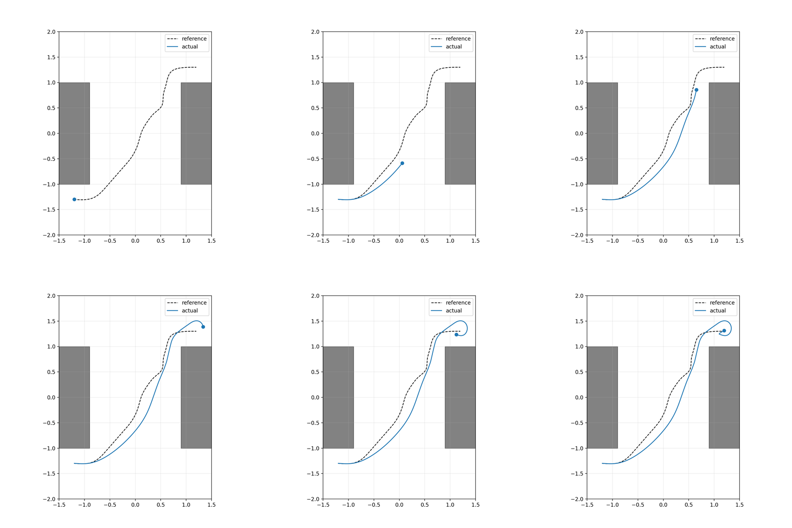
The controller follows the spline using the estimated pose, not the true one. It combines feed-forward (where the reference is heading) with feedback (how far off we are), then turns that into left and right wheel forces.
The commanded velocity is the spline's velocity plus a correction toward the reference, capped at 0.5 m/s:
$$v_{\text{cmd}} = \dot x^*(t) + K_p\,\big(x^*(t) - \hat x\big)$$Rotated into the body frame, its forward part sets a force \(F\) and its angle \(\varphi\) sets a turning torque \(\tau = k_\varphi \varphi - k_\omega \omega\). Inverting the wheel model from earlier splits these into wheel commands, clipped to \(\pm 1\) N:
$$u_{l} = \frac{F}{2} - \frac{\tau}{b}, \qquad u_{r} = \frac{F}{2} + \frac{\tau}{b}$$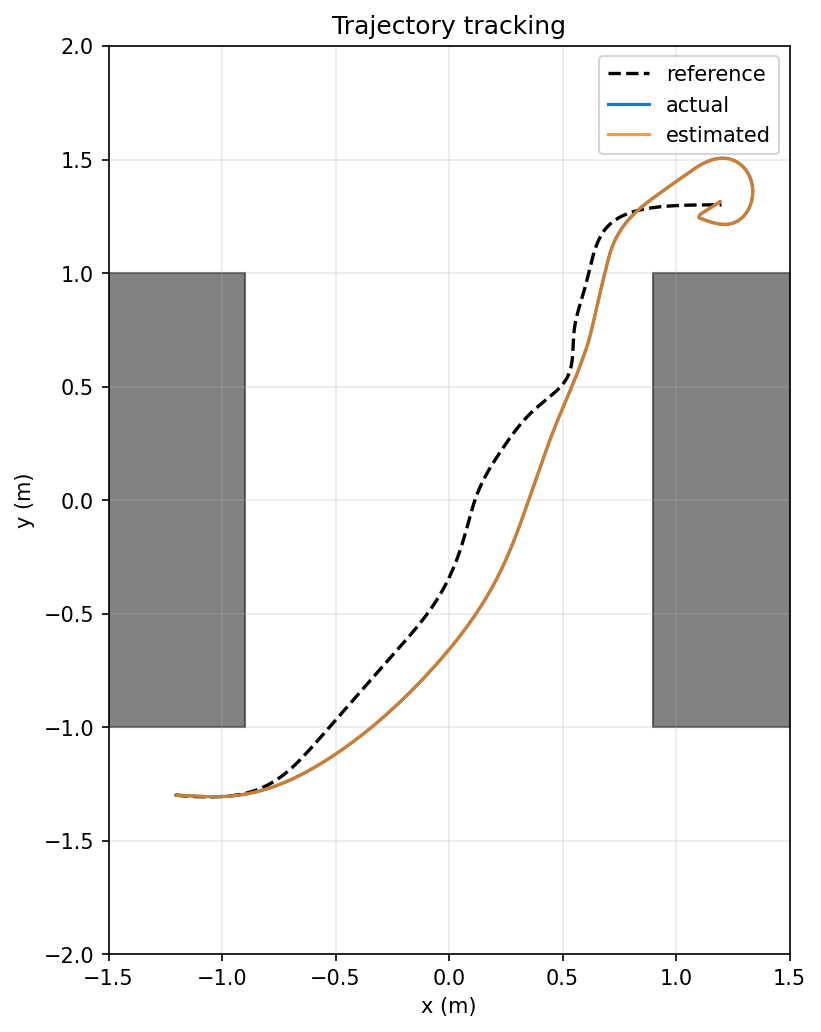
Moving obstacles
The same planner can run in a loop: plan one second ahead, execute a small slice, then replan from wherever the robot actually is. That lets it dodge an obstacle that sweeps back and forth across the gap. Across the full run the robot never came closer than 0.25 m to it, comfortably above the 0.15 m safety floor.
The obstacle follows \(x_{\text{obs}}(t) = [\,0.5\sin(\pi t),\ 0\,]\) with radius 0.4 m. Two terms in the band's cost change: the time term holds each plan to the 1-second horizon, and clearance is checked against where the obstacle will be when the robot reaches each waypoint:
$$J_{\text{time}} = \gamma_t \Big(\textstyle\sum_k \Delta t_k - T_H\Big)^2$$ $$d_k = \big\lVert p_k - x_{\text{obs}}(t_{\text{now}} + t_k) \big\rVert - r_{\text{obs}}$$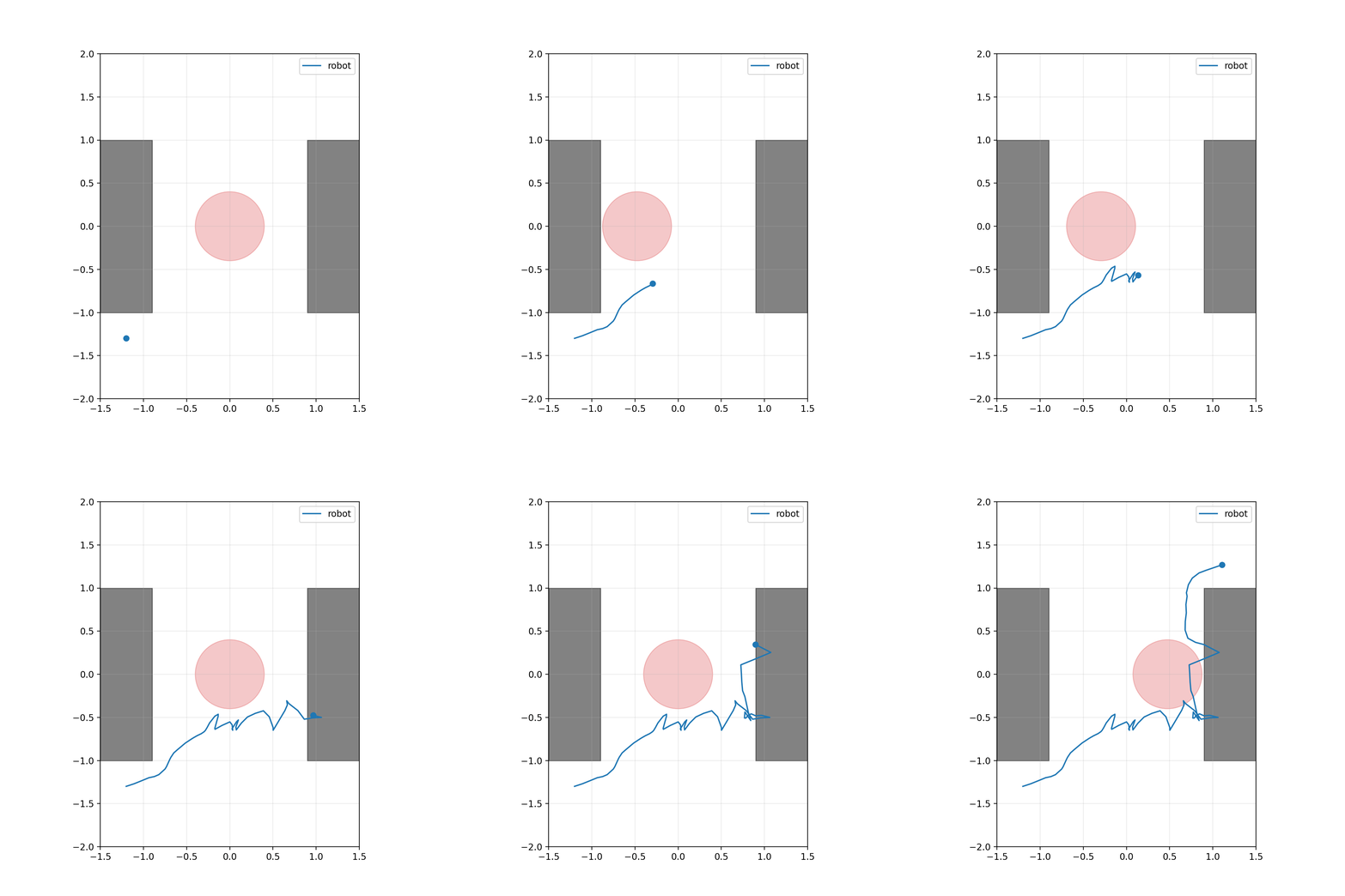
Chaining goals
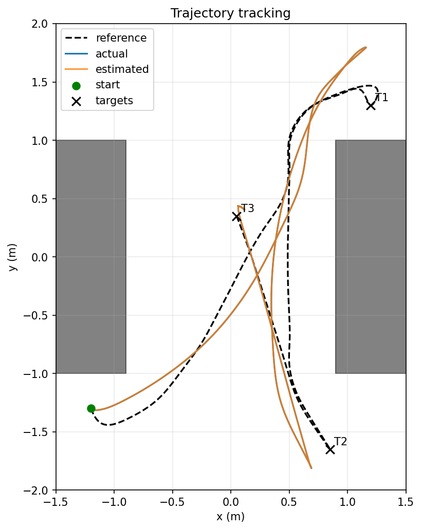
Because the spline handles any set of waypoints, chaining several goals was mostly a matter of stitching plans together. The robot visits three targets in sequence, though the sharp reversals push the wheels into saturation and the tracking error grows in the tight turns. Smarter time-scaling around corners is the obvious next step.